Example: approximating derivatives using DG
RefElemData and MeshData can be used to compute DG derivatives. Suppose $f$ is a differentiable function and the domain $\Omega$ can be decomposed into non-overlapping elements $D^k$. The approximation of $\frac{\partial f}{\partial x}$ can be approximated using the following formulation: find piecewise polynomial $u$ such that for all piecewise polynomials $v$
\[\int_{\Omega} u v = \sum_k \left( \int_{D^k} \frac{\partial u}{\partial x}v + \int_{\partial D^k} \frac{1}{2} \left[u\right]n_x v \right)\]
Here, $\left[u\right] = u^+ - u$ denotes the jump across an element interface, and $n_x$ is the $x$-component of the outward unit normal on $D^k$.
Discretizing the left-hand side of this formulation yields a mass matrix. Inverting this mass matrix to the right hand side yields the DG derivative. We show how to compute it for a uniform triangular mesh using MeshData and StartUpDG.jl.
We first construct the triangular mesh and initialize md::MeshData.
using StartUpDG
using Plots
N = 3
K1D = 8
rd = RefElemData(Tri(), N)
VXY, EToV = uniform_mesh(Tri(), K1D)
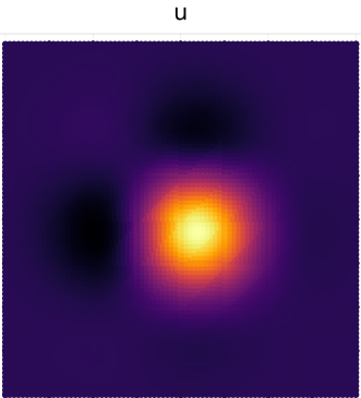
md = MeshData(VXY, EToV, rd)We can approximate a function $f(x, y)$ using interpolation
f(x, y) = exp(-5 * (x^2 + y^2)) * sin(1 + pi*x) * sin(2 + pi*y)
(; x, y) = md
u = @. f(x, y)
or using quadrature-based projection
(; Pq ) = rd
(; x, y, xq, yq ) = md
u = Pq * f.(xq, yq)
We can use scatter in Plots.jl to quickly visualize the approximation. This is not intended to create a high quality image (see other libraries, e.g., Makie.jl,VTK.jl, or Triplot.jl for publication-quality images).
(; Vp ) = rd
xp, yp, up = Vp * x, Vp * y, Vp * u # interp to plotting points
scatter(xp, yp, uxp, zcolor=uxp, msw=0, leg=false, ratio=1, cam=(0, 90))
Both interpolation and projection create a matrix u of size $N_p \times K$ which contains coefficients (nodal values) of the DG polynomial approximation to $f(x, y)$. We can approximate the derivative of $f(x, y)$ using the DG derivative formulation
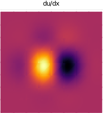
function dg_deriv_x(u, rd::RefElemData, md::MeshData)
  (; Vf, Dr, Ds, LIFT ) = rd
  (; rxJ, sxJ, J, nxJ, mapP ) = md
  uf = Vf * u
  ujump = uf[mapP] - uf

  # derivatives using chain rule + lifted flux terms
  ux = rxJ .* (Dr * u) + sxJ .* (Ds * u)
  dudxJ = ux + LIFT * (.5 * ujump .* nxJ)

  return dudxJ ./ J
end
We can visualize the result as follows:
dudx = dg_deriv_x(u, rd, md)
uxp = Vp * dudx
scatter(xp, yp, uxp, zcolor=uxp, msw=0, leg=false, ratio=1, cam=(0,90))
Plots of the polynomial approximation $u(x,y)$ and the DG approximation of $\frac{\partial u}{\partial x}$ are given below
 ⠀
⠀