Background
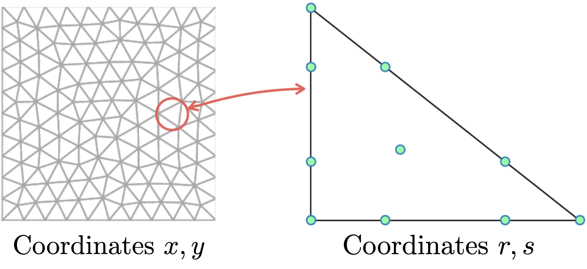
Most high order finite element methods rely on a decomposition of a domain into a mesh of "elements" (e.g., triangles or quadrilaterals in 2D, hexahedra or tetrahedra in 3D). Each "physical" element in a mesh is assumed to be the image of single "reference" element under some geometric mapping. Using the chain rule and changes of variables, one can evaluate integrals and derivatives using only operations on the reference element and some geometric mapping data. This transformation of operations on all elements to a single reference element make finite element methods efficient.
We use the convention that coordinates on the reference element are $r$ in 1D, $r, s$ in 2D, or $r, s, t$ in 3D. Physical coordinates use the standard conventions $x$, $x, y$, and $x, y, z$ in 1D, 2D, and 3D.
Derivatives of reference coordinates with respect to physical coordinates are abbreviated, e.g., $\frac{\partial r}{\partial x} = r_x$. Additionally, $J$ is used to denote the determinant of the Jacobian of the reference-to-physical mapping.
Assumptions
We make a few simplifying assumptions about the mesh:
- meshes are conforming (e.g., each face of an element is shared with at most one other element).
- the geometric mapping from reference to physical elements is the same degree polynomial as the approximation space on the reference element (e.g., the mapping is isoparametric).
Initial experimental support for hybrid, cut-cell, and non-conforming meshes in two dimensions is also available. Please see the corresponding test sets test/hybrid_mesh_tests.jl, test/cut_mesh_tests.jl, and noncon_mesh_tests.jl for examples.
Code conventions
StartUpDG.jl exports structs RefElemData{Dim, ElemShape, ...} (which contains data associated with the reference element, such as interpolation points, quadrature rules, face nodes, normals, and differentiation/interpolation/projection matrices) and MeshData{Dim} (which contains geometric data associated with a mesh). These are currently used for evaluating DG formulations in a matrix-free fashion. These structs contain fields similar to those in Globals1D, Globals2D, Globals3D in the NDG book codes.
We use the following code conventions:
- variables
r, s, tandx, y, zcorrespond to values at nodal interpolation points. - variables ending in
q(e.g.,rq, sq,...andxq, yq,...) correspond to values at volume quadrature points. - variables ending in
f(e.g.,rf, sf,...andxf, yf,...) correspond to values at face quadrature points. - variables ending in
p(e.g.,rp, sp,...) correspond to equispaced plotting nodes. Dr, Ds, Dtmatrices are nodal differentiation matrices with respect to the $r, s, t$ coordinates. For example,Dr * f.(r, s)approximates the derivative of $f(r, s)$ at nodal points.Vmatrices correspond to interpolation matrices from nodal interpolation points. For example,Vqinterpolates to volume quadrature points,Vfinterpolates to face quadrature points,Vpinterpolates to plotting nodes.- geometric quantities in
MeshDataare stored as matrices of dimension $\text{number of points per element } \times \text{number of elements}$.
Differences from the codes of "Nodal Discontinuous Galerkin Methods"
The codes in StartUpDG.jl are based closely on the Matlab codes from the book "Nodal Discontinuous Galerkin Methods" by Hesthaven and Warburton (2008) (which we will refer to as "NDG"). However, there are some differences in order to allow for more general DG discretizations and enforce certain mathematical properties:
- In NDG,
Fmaskextracts the interpolation nodes which lie on a face. These nodes are then used to compute interface fluxes. However, in StartUpDG.jl, we interpolate nodal values to values at face quadrature points viard.Vf * u. These operations are equivalent if the interpolation nodes which lie on a face are co-located with quadrature points. Similarly, in NDG, theLIFTmatrix maps face nodal points to volume nodal points. InStartUpDG.jl, therd.LIFTmatrix maps from face quadrature points to volume nodal points. - in NDG, there are connectivity arrays
vmapMandvmapP, which directly retrieve interface values from arrays of nodal values. InStartUpDG.jl, face interpolation nodes are not guaranteed to be co-located with face quadrature nodes, so we do not providevmapMandvmapP. Instead, we expect the user to compute face values and use themd.mapM,md.mapParrays to access interface values. - in NDG, the mass matrix is computed exactly using the formula
M = inv(VDM * VDM'), whereVDMis the generalized Vandermonde matrix evaluated at nodal interpolation points. InStartUpDG.jl, the mass matrix is computed using quadrature. These are equivalent if the quadrature is exact for the integrands in the mass matrix (e.g., degree $2N$ polynomials for triangular or tetrahedral elements). - in NDG, the geometric terms
rx, sx, ry, sy, ...are computed and stored. InStartUpDG.jl, the scaled geometric termsmd.rxJ, md.sxJ, md.ryJ, md.syJ, ...are computed, which enable us to enforce the metric identities on curved meshes. Similarly, NDG providesFscale = sJ ./ J(Fmask, :), whileStartUpDG.jlonly providesmd.Jf, which is equivalent tosJ.Fscale, as well as the NDG geometric terms and can be recovered by dividing bymd.J.
Internally, NDG uses arrays EToE and EToF to compute the interface connectivity array mapP. StartUpDG.jl uses instead a face-to-face connectivity array FToF. However, EToE, EToF, and FToF are not typically required for the matrix-free explicit solvers targeted by this package.